Different views of the brain
- Coronal view: View after cutting the face off.
- Sagittal medial view: Cutting brain from the sides into the middle.
- Lateral Sagittal view: Take the skull off.
- Axial view: Look from the top after cutting off a piece.
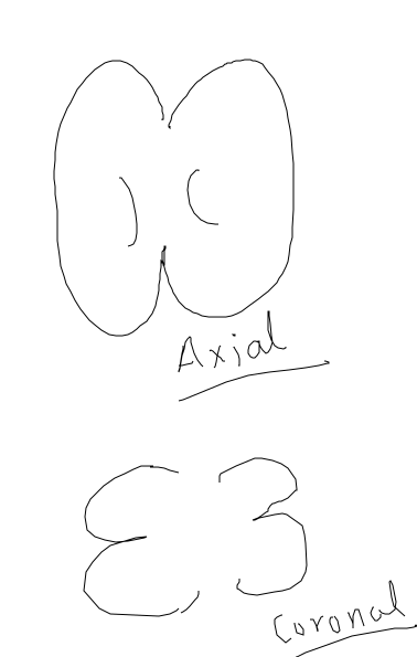
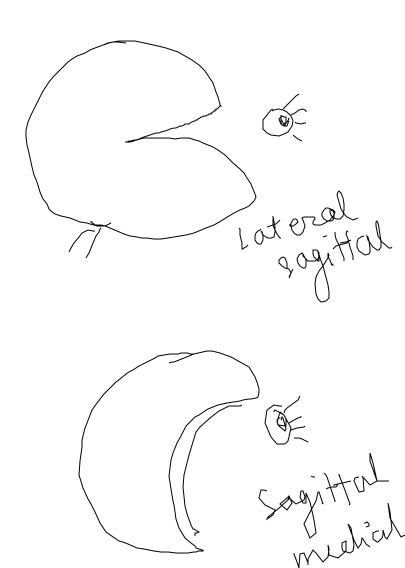
- Sulca: Bottom of cortical folds
- Gyrus: Top of cortical folds
Different Imaging Techniques
Anatomical Imaging
- Axial slices are 2D representations.
- Making multiple axial slices –> 3D representation of the brain
- Slices can be separated by some space.
- Voxel: Spatial Resolution of 3D fMRI representation
- In plane resolution: Pixel of 2D slice
- Going very high resolution has a downside that the blood flow in the brain decreases SNR in our images.
- Dead brains can be imaged with very high resolution.
- Spatial Resolution depends on pixel and separation.
- Example: 1 mm isotropic , 1*1*1 mm, 176 slices, 5 min : Example of how fMRI are defined.
Functional Imaging
- Add temporal resolution to anatomical data. The 3D representation taken in different time steps. The time between two images is known as repetition time. Generally it’s 2 seconds.
- 2 seconds vs 5 minutes: Sacrifice spatial resolution; Generally it’s 3*3*3 and 30 slices.
- 27 anatomical voxels compared to 1 anatomical voxel.
fMRI Time-course
Hemodynamic Response function(HRF)
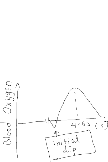
- The brain has a high oxygen level in the region after activity. There is a undershoot after some time after peak.
- This is the general HRF used to process fMRI data.
- HRF looked in baby mice was found to be very slow. Mostly for adults and general experiments, the standard HRF is used. α is the time to peak which is also called Human Anatomical Lag and β is the peak level. α is fixed generally and we solve for β.
- Variability in α is smaller than β. So, even if we have different values of α across different brain regions, we neglect it for general experiments.
- 2 seconds time in Functional fMRI is only useful for the HRF just drawn above. So, we need to have it small to resolve the peak of HRF.
- Big blood vessels at smaller scale can turn into noise around the given voxel.
- Astrocyte in early visual cortex have 1:1 relation with neurons and can be used to get same spatial resolution as the neural activity.
- The shape of HRF and α is something we take as prior knowledge.
- Negative β is when given the input signal, the blood oxygen level decreases relative to normal case.
- BLOD signal [ Actual signal ] Unit:
- %SC[Signal Change]: Relative to normal, how different is BLOD signal in the experiment.
General Linear Model (GLMs)
- Boxcar regressor : Box shaped signal multiplied by HRF signal.
- Single GLM with multiple regressors.
- β values per voxel is taken. So, it’s a single 3D image of brain with different beta. If you have multiple inputs, there will be multiple β values. Or you can have β count = no of runs * no of conditions
- If you just have β image and don’t know how many runs did β came from one signal’s full time snapshot, then it’s ruined data. You need information about how the data’s obtained as well.
Noise:
- e.g Sneezing where the whole brain breaks and has spike in response at that time. People can move their head and these noise make the signal unusual or crazy.
- Solution: To handle this, put an impulse regressor with single time-point with same height as the data’s amplitude. So, this regressor explains whole information and no other regressors don’t take into account of it since the first one explains it by default.
Steps in data analysis:
- Raw data: Scanner in DICOOM format.
- Preprocessing: Motion correction of head, smoothing etc.
- Modeling: Comparing the data with your prior and your input. The output will be β values.
Univariate analysis
Answer How much is neural activity?
- Need to first answer Where question first.
- Average/Any other metric of all voxels in the region of interest. The difference of betas between different ROIs is known as contrast value.
- Even though we can’t ask contrast value’s quantity means but we can see if there is a difference in contrast value across different persons.
- So, this can tell only the consistency of the data using t-test.
Answer Where is the neural activity?
- You don’t know where you should find the activity.
- Now for every voxel, contrast value is calculated obtaining a 3D map of brain of contrast values.
- Know the variance of each voxel data from initial beta calculation analysis.
- t-map has value at every voxel which is size of contrast value compared to the unexplained variance used in calculating initial beta.
- Now find big values in t-map using thresholding. Generally threshold is <0.001. Now, we generally get contiguous voxels as our region. Now, we can use this to answer How much question now.
Whole Brain Group Analysis
ID: 827294d7-0097-4aac-a0fc-9b29c6b836d7
- Align brains
- How do you know which voxels are the same in different person?
- MNI-152 brain. Average anatomical template of brain.
- Most normalizing images are the functional ones since they are the ones that need aligning. So, we register functional mapping to it’s analytical image and then map it to anatomical template. The first mapping is pretty easier compared to the second. These steps are known as Registration and Normalization.
- Figure out best fit between the images using affine transformations and calculate which point in anatomical brain is similar in the template. This is not perfect. For higher regions, the alignment is very poor. Most easier to map is V1 and it’s also only 40% accurate.
- FMRI Hyperalignment and Functional ROI are other steps that can be added to solve the problem with the mapping talked above.
- Statistics over people
- Contrast value across different person and for specific region, we can average contrast value for all persons. Now, for every contrast map across persons, t-map by using variability across persons. Then, threshold t-map. This statistics over people is known as Second level Analysis/Random Effects Analysis. For this analysis, the number of people will define the robustness of experiment.
Multivariate analysis
- Comparing to the univariate analysis, where we draw different betas across voxels distributed in space for different conditions, we know which voxels activate to which signal. This was the previous way of analysing our signal.
- Now, we can represent all voxels as dimension of multidimensional space. If we have 12 voxels, it’s 12 dimensions. But, we can’t observe spatial relation between voxels though. We cannot do such analysis with all voxels though.
- Which voxels to choose?
- Advantages
- Classification
- Similarity Analysis using Distance
Relationship
- Brain region in superior temporal gyrus. “TO RUN” vs “THE ROCK”, the words have different activity in this region. What is this about? Verbs vs Nouns or Objects in motion vs Stationary Objects. This is about testing the question.
- Experimented with more pair of words drawn from four classes:
- Verbs with motion : “To run”
- Verbs without motion: “To think”
- Nouns with motion: “The Tiger”
- Nouns without motion: “The Rock”
- Experimental data:
- Prior Analysis
- Time series analysis
- 1 regressor per condition per run
- 8 runs in the experiment
- 4 different conditions
- Total of 32 betas for each voxel found
- Prior Analysis
- Univariate analysis:
- Contrast Image
- Running vs Rock in some person which is above the threshold. This is the region of interest.
- We do it for different persons. Now, we say “STG” is actually where the differences occur.
- Now , univariate question “How much” ?
- Averaging over runs. Now, we can have “RUN” vs “ROCK” difference of betas. We can do it similarly for all sets of differences between conditions: “nouns vs verbs” or “motion vs stationary”. The differences should be larger on the criteria that we intend to find.
- Now, though you find a distinction, there might be different set of differences between the nouns you are taking as well. e.g. “The Tiger” and “The Rock” might be interpreted into different classes as well. So, this goes on. Philosophical debate on “non-zero” responses in all conditions. What does it mean?
- Contrast Image
- Multivariate analysis:
- Now, In ROI of around 80 voxels, 8 beta values per run in each condition.
- In each subject, this can be plotted separately. “Leave one out” beta classification with two boundaries: “ROCK and TIGER” vs “RUNNING” and “THINKING”. Now, can you classify between nouns and verbs inside the multivariate analysis. You plot seven betas thus and make boundary. Finally you average all those results.
- Think about it : If we see difference in univariate analysis, there will
surely be difference in multivariate analysis as well. But, even if there is
no difference in univariate analysis , there might be difference that could
be observed in multivariate analysis.
- About the example: We know “NOUNS” and “VERBS” were distinctly separated in univariate analysis. So, we can separate that boundary clearly in multivariate as well. But, can we separate “MOTION NOUNS” vs “STATIONARY NOUNS” and similarly for verbs is a question that can be answered by multivariate analysis only.
- Relative information is one that is available in multivariate analysis only.
- Classification accuracy in verbs and nouns can now be found. This can show now that the “STG” region also has more information to classify between the nouns or the verbs if the difference in accuracy is relatively high.
Finding useful region
- ROI Identification in multivariate analysis. Where question
- Commonly known as Feature Selection in ML where the voxels are the features.
- Choosing Features:
- Anatomy : e.g Amygdala
- Functional area e.g. SFG [Contiguous regions]
- Functional PCI-n : Number of voxels in any direction.
- Why choose voxels?
- Relevant unit of analysis
- Local region: Region with certain characteristic that carries out a functional work or encode certain feature space.
- Functionally defined network: Even if regions are not contiguous, they might have functional correlation. e.g. Regions in opposite hemispheres.
- Statistical Reasons
- By adding noise i.e. not useful voxels to the total space, we will have low SNR: so lower quality of analysis. Thus, we choose only a number of voxels for our analysis.
- Noise also can create significant differences in signal. So, if we know relevant voxels, we can ignore voxels that do not help in our analysis. It prevents over-fitting in general.
- Relevant unit of analysis
Classification
ID: acb8de53-9d7b-4375-add1-d7a5dd14ba8e
- Example:
- Show female sad faces and happy faces. Now, classify them each run, each individual and finally average them. This is the first step.
- We want to know if the emotions in real are making the difference in signal, if you show male sad faces and happy faces; if the original boundary generalizes to male faces as well, you know that emotions is encoded by that region.
- For number of runs required per person, there is not a fixed number but it’s generally good to have more runs.
- In binary classification NEVER have unequal number of images in each run. Don’t let bias get into it.
- In data, we need to take care of the additional information present in the data as well.
- The overall output was that there was proof for certain region which classified general images but could not generalize to cartoon images. And there was proof for different region that could generalize to both regions. So, one implies only facial information present whereas the other implies more to all regions.
- Generally, you look for main information by comparing different brain regions. If you see a likely result from that classification, then there is a hierarchical number of analyses that can be done on top of that result.
- Do positive control such as : Rotation of images and so on. You can do negative control as well.
- Near Generalization : Generalizing to man faces in this case.
- Far Generalization: Generalizing to cartoon faces as well.