4 minutes
R Programming 105- Unsupervised Learning
K Means Clustering
res <- kmeans(x,
              centers = num,
              nstart = num,
              iter.max = 20)
res$cluster # gives the cluster number for each data point
print(res) # prints cluster means, cluster, sum of squares by cluster and so on.
-
Arguments
- Centers is the number of clusters to make.
- Nstart is used to run algorithm multiple times to improve the odds of the best model.
- Iter.max is used to set the number of steps to do when creating each clusters.
-
Visualizing output
plot(points,
     col = res$cluter,
     main = "title of the plot")
-
Best number of clusters
-
Scree Plot
Plot within ss vs number of clusters to find the elbow of the plot. Choose that number of clusters to create k-means. This plot is known as scree plot. This is useful since trial and error is not the best approach.
library(purrr)
withinss <- map_dbl(1:20, function(k) {
  model <- kmeans(x = df, centers = k)
  model$tot.withinss
    })
elbow_kmeans <- data.frame (
  k = 1:20,
  withinss = withinss
    )
# 1:20 is the number of clusters which you seem to find best fit from.
# When plotting put a scale so that it's easier to find k since you don't want decimal valued k.
ggplot(elbow_kmeans, aes(k, withinss)) +
  geom_line() +
  scale_x_continuous(breaks = 1:20)
This gives you a df which has number of clusters “k” vs Within sum of squares “withinss”. Plotting these you get a scree plot.
-
Silhouette width
- Within cluster distance : To other cluster. C(i)
- Closest Neighbor distance : To other clusters point. N(i)
-
Formula
\[ s(i)=\left\{\begin{array}{ll}1-C(i) / N(i), & \text { if } C(i)<N(i) \\\ 0, & \text { if } C(i)=N(i) \\\ N(i) / C(i)-1, & \text { if } C(i)>N(i)\end{array}\right. \]
-
Analysis
1: Well matched to cluster 0: On border between two clusters -1: Better fit in the neighboring clusters.
library(cluster)
pam_values <- pam(df, k = sth)
pam_values$silinfo$widths # get silhouette widths
pam_values$silinfo$avg.width # get avg of all s(i)
plot(silhouette(pam_values))
-
Choosing K with this s(i)
The value of K with max value of s(i) is to be chosen for creating the clusters.
-
Hierarchical Clustering
- Number of clusters is not known ahead of time
- Similarity measured via some kind of distance metric.
hclust(dist(x))
summary(hclust_obj)
-
Dendrogram
To analyze we can make dendrograms to understand the result properly.
plot(hclust_obj)-
Coloring dendrograms
Based on height parameter passed as “h” or num of clusters “k”, we can color the dendogram for cleaner representations.
library(dendextended)
dend_obj <- as.dendogram(hclust_obj)
colored_plot <- color_branches(dend_obj, k = num)
colored_plot <- color_branches(dend_obj, h = num)
-
-
Finding a subtree
Cut a hierarchical subtree
cutree(hclust_obj, h = sth) # height of clusters
cutree(hclust_obj, k = sth) # k is no of clusters
-
Linking Clusters
- Complete: Pairwise similarity between all observations
- Single: Smallest of similarities between all observations
- Can create unbalanced trees
- Average: Average of similarities to link clusters
- Centroid: Find similarity between centroids
- Inversions of clusters and so not used mostly.
-
Methods
In this method, we cluster based on linkage methods to choose from and form clusters hierarchically. We start with the minimum distanced points and make them 1st cluster. Then find linkage distance between points in cluster 1 and rest of the points. If rest of the points have smaller distances, they may form a different cluster. Or else you can have another point added to the 1st cluster to form hierarchical 2nd cluster.
-
Complete Linkage
When we have more than two objects and intend to find the distance between them, we can find that using linkage method which takes the maximum of that point to other points as closeness metric.
max(dist(obj_1, obj_2), dist(obj_2, obj_3))
-
Single Linkage
min(dist(obj_1, obj_2), dist(obj_2, obj_3))
-
Average Linkage
mean(dist(obj_1, obj_2), dist(obj_2, obj_3))
-
Using the methods
hclust(d, method = "complete")
hclust(d, method = "average")
hclust(d, method = "single")
-
Issues and Solutions
- Normalize features since scales will be different.
scale(df) # normalizes df
PCA
prcomp(x = data,
       scale = FALSE,
       center = TRUE)
The dataframe is similar to other cases as well.
-
Arguments
- scale: Column sd used to scale the data if TRUE
- center: Column means to center the data if TRUE
- rotation: Directions of PCA vectors in terms of original variables. Define new data in terms of original PCAs.
-
Interpreting Results
summary(pca_obj) # gives the output about how influential are principal components-
Creating Biplot
biplot(pca_obj)
-
Scree Plot
variance <- pca_obj$sdev ^ 2
pve <- variance / sum(variance)
plot(pve)
-
Plotting of Variance Explained
plot(pve)
plot(cumsum(pve))
These two different kind of plots help to find the elbow.
-
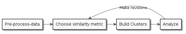
Cluster Analysis
-
Overall Flow
-
Distance Metrics
-
Categorical Data
Jaccard’s index = Intersection / Union Distance = 1 - J.I It checks how many categories are similar between observations and how many there could be.
dist(df, method = "binary")When you have multiple categories and you want to convert them to binary variables as 1 and 0.
library(dummies)
dummy.data.frame(df_name)
-
Backlinks
801 Words
2020-10-09 00:00 +0545